Getting Tied Up in Knot Theory

This post draws inspiration from the Veritasium YouTube video, The Insane Math Of Knot Theory. If you haven’t seen it, I highly recommend checking it out Here.

Trefoil Knot

Imagine taking a piece of string, tangling it in the most complex way possible, and then joining its ends together. How can you determine if this knot is truly unique or if it can be transformed into something simpler?

This fundamental question lies at the heart of knot theory, one of mathematics’ most intriguing branches.

What is Knot Theory?

Definition and Basic Concepts

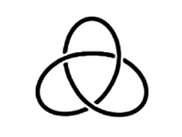
A mathematical knot is fundamentally different from the everyday knots we tie in shoelaces or ropes. In mathematics, a knot is a closed loop embedded in three-dimensional space that cannot be untangled without cutting. Think of it as a piece of string with its ends joined together, creating a continuous loop that might be twisted or tangled in various ways.

  At its core, knot theory focuses on mathematical knots. Unlike those we tie in our shoelaces, mathematical knots are closed loops without any free ends. 

The primary goal of knot theory is to understand and categorize these knots based on their properties. Mathematicians examine invariants—features that remain consistent even as a knot is stretched, twisted, or morphed (as long as it isn’t cut or unlooped).

Invariants are crucial for distinguishing one knot from another and for uncovering connections between knots and various fields of mathematics and science.

Tip: Did you know? The oldest known knot is the square knot, used as early as 3500 B.C. in ancient Egypt!

To date, approximately 352,152,252 unique knots have been identified, each possessing distinct properties and characteristics.

How Can We Distinguish Knots?

This leads us to a fundamental question: How can we distinguish one knot from another?

To explore this, you might try an experiment. Take a piece of string or an extension cord, tie it into a knot, and then join the ends together to form a closed loop. Now, attempt to transform a trefoil knot into a different knot. You’ll likely find this task quite challenging.

Eventually, you may conclude that the two knots are fundamentally different. But how can we turn this practical exercise into a mathematically precise process?

Blue Trefoil Knot Animated

Reidemeister’s Solution

Enter Kurt Reidemeister. He introduced three specific techniques for manipulating knots, providing mathematicians with a systematic framework for their analysis. Instead of relying solely on trial and error, Reidemeister’s moves allow us to examine knots methodically. If no combination of these moves can transform one knot into another, we can confidently assert that the two knots are distinct.

Kurt Reidemeister

The three Reidemeister moves are intuitive and resemble a kind of mathematical dance: a twist, a poke, and a slide. These basic operations can be performed on a knot diagram to alter its structure. By applying these moves, we can determine whether a knot is unique or merely a variation of another.

The Three Reidemeister Moves

Type I (Twist): Creates or eliminates a twist in a strand.
Type II (Poke): Moves one strand completely over another.
Type III (Slide): Slides a strand past a crossing.

\text{Knot Equivalence} \iff \exists \text{ sequence of Reidemeister moves}

However, this method raises critical questions:

Does it guarantee that we can distinguish every two knots?
How can we ensure that we have tried every possible combination of Reidemeister moves?
What if there is a clever sequence of moves that can completely unravel the knot, which we have overlooked?

These inquiries point to the deeper challenges within knot theory and highlight our continuous pursuit of understanding knots better.

The First Real Tool to Solve Knots

Reidemeister moves are just the beginning of knot theory. A significant advancement came in the form of tricolourability.

For a knot diagram to be tricolourable:

Every section of the knot must be filled with three distinct colours.
At each crossing, the strands must be either all the same colour or all different colours.

For example, the unknot is not tricolourable because it has only one strand to colour, thus violating the first condition.

a + b \equiv 2c \, (\text{mod } 3) \text{ with } a, b, c \in \{0, 1, 2\}.

Tricoloring

These values correspond to the colours we might assign to the strands, such as red, green, and blue. You can experiment with different combinations to see how this equation provides a structured way of colouring the strands.

Tricolourability is a knot invariant: a property that remains unchanged during ambient isotopy or any allowed moves (except for cutting the knot, which is not permitted in topology).

Knot invariance directly addresses our original question. If one knot is tricolourable while the other is not, it confirms that they are indeed different, as there’s no way to transform one into the other.

Advanced Knot Classifications

Now that we can classify knots into two groups—tricolourable and non-tricolourable—we realize this isn’t the end. Consider the figure-eight knot and the unknot; neither is tricolourable, yet they are clearly different knots.

It turns out tricolourability is just a subset of a broader concept known as prime-colourability. Instead of three colours, we can utilize any prime number of colours to extend our classification system.

The corresponding mathematical expression is:

a + b \equiv 2c \, (\text{mod } p)

From Reidemeister moves and tricolourability to prime-colourability and the concept of knot determinants, we’ve developed a comprehensive framework for tackling our original question. While challenges persist—such as distinguishing mirror images or highly complex knots—we have made remarkable progress in knot theory.

Knot Diagrams

A knot diagram is a two-dimensional representation of a knot, depicting how the strands cross over and under each other. These diagrams are essential for visualizing and analyzing knots.

Knot Diagram

Crossing

Crossing refers to the points in the diagram where one strand passes over or under another. Understanding crossings is crucial for analyzing and manipulating knots.

Reidemeister Moves

These three simple manipulations (twists, pokes, and slides) are applicable to knot diagrams, allowing mathematicians to alter the diagram without affecting the knot’s fundamental structure.

Invariants

An invariant is a property of a knot that remains unchanged regardless of how the knot is stretched, twisted, or deformed (as long as it isn’t cut or untied). Invariants are vital for classifying knots and determining whether two knots are equivalent.

Some important invariants include:

Alexander Polynomial: Introduced in 1928, this tool assigns a polynomial to each knot, aiding in classification.

\Delta_K(t) = a_0 + a_1t + a_2t^2 + ... + a_nt^n

Example for the trefoil knot:

\Delta_{\text{trefoil}}(t) = t^2 - t + 1

Jones Polynomial: Discovered in the 1980s, this invariant has significant connections to quantum mechanics. It fundamentally changed the field by providing new ways to classify knots.
Crossing Number: The minimum number of crossings required to draw a knot diagram.

  Fun Fact: The **Celtic knot**, known for its intricate weaving patterns, symbolizes eternity, unity, and interconnectedness. 

These invariants help differentiate knots that may seem similar but are fundamentally different.

Links

A link is a collection of multiple knots that are intertwined. While a single knot is a closed loop, a link consists of two or more loops that may be knotted together.

Borromean Rings

A famous example of a link where three loops are connected in such a way that no two loops are directly linked, yet all three are inseparable.

Brunnian Links

Brunnian Link

These links demonstrate the property that removing any one loop causes the others to disassemble. Links introduce an additional layer of complexity to knot theory, incorporating interactions among multiple knots.

The History of Knot Theory

Knots have been integral to human life for thousands of years. Early humans employed knots for hunting, building shelters, and creating tools. Sailors relied on knots to secure sails and anchor ships. Examples such as the bowline, clove hitch, and reef knot have been passed down through generations.
Table of Knots

The Birth of Knot Theory

In the 1860s, Scottish physicist William Thomson (Lord Kelvin) proposed a novel idea: atoms might be tiny, knotted vortices in a universal ether. Though this theory was discredited, it sparked interest in the mathematical study of knots.

Mathematician Peter Guthrie Tait began cataloging knots based on complexity and crossings, which laid the groundwork for modern knot theory.

The 20th Century: Knot Theory Takes Off

In the early 1900s, knot theory became part of topology, the study of shapes and spaces. Mathematicians concentrated on invariants—properties that do not change when a knot is stretched or twisted.

In 1928, James Waddell Alexander introduced the Alexander polynomial, a key instrument in distinguishing between knots. This marked a breakthrough in the systematic classification of knots.

Knot Theory Meets Modern Science

In the late 20th century, knot theory found applications in biology, chemistry, and physics. Researchers discovered that DNA forms knots and that chemists employed knot theory to understand intricate molecules.

In the 1980s, mathematician Vaughan Jones discovered the Jones polynomial, linking knot theory to quantum mechanics. This discovery opened doors to research in string theory, particle physics, and black holes.

Getting Tied Up in Knot Theory - A Fun Overview